Huffman Compression

Data compression is a process of modifying the representation of some information so that it can be stored using less data. Storing and transmitting data is expensive in large quantities, making an optimal compression (one which minimizes storage size) extremely valuable. In this post we will learn how to quantify data information-theoretically¹, and how to get an optimal compression with optimal speed.

The ratio of concepts and definitions to prose is pretty high in this post, but I try to ameliorate that with examples and alternate descriptions. Assuming a bit of familiarity with binary and ASCII, nothing here should be too dificult to understand. It’s okay to skim over some of the equations, there won’t be a test at the end.

Entropy: Quantifying Information

Let $\Omega$ be some set, and $P = \{p_i,\, i\in \Omega\}$ be the probability distribution over $\Omega$, i.e. the frequency with which each element of $\Omega$ occurs. The entropy of $\Omega$ is a measure of how structured (non-uniform) $P$ is. So for example, the uniform distribution (where $\forall p_i \in \Omega,\, p_i = \frac{1}{|\Omega|}$) is the least structured, and the lowest entropy. Conversely, the distribution where $p_{i_0} = 1,\, p_i = 0 \, \forall i \neq i_0$, is the most structured, and has the most entropy.

More intuitively, entropy can be thought of as a measure of how uncertain you are about a random choice from $\Omega$, using $P$. With a set of minimal entropy (one with a uniform distribution), you can do no better than a random guess. But on a set where one element has a probability $1$ of occurring, and the rest have probability $0$, you can be certain that the next element to occur will be that one with probability $1$.

Formally, the entropy of $P$ is given by $H(P) = - \sum\limits_{i \in \Omega} p_i \cdot \log(p_i)$.

Fact: $0 \leq H(P) \leq \log(|\Omega|) = H(P_{uniform})$.

Applying Entropy

Remarkably, a choice from $\Omega$ contains $H$ bits of information per element.

Take $\Omega = \{A, B, ..., Z\}$. $\log(|\Omega|) = \log(26) = 4.17$. Then naively we can represent the alphabet using 5 bits. Perhaps $A = 00000, B = 00001, ..., Z = 11001$. Now we can imagine using this coding on a text file we wrote (of only these 26 characters). The size of this file (ignoring metadata and whatever) is 5 bits per character $\times$ the number of characters.

Already you might see that this is suboptimal. With 5 bits, you can represent as many as 32 characters ($2^5 = 32$), so we could add 6 more chacters to our alphabet without using any extra data per character. This is an improvement, but still we’re restricting ourselves. What if we used a variable number of bits per character?

Coding

A coding $C$ of $\Omega$ is a unique mapping between the elements of $\Omega$ and a set of binary strings. The mapping $A = 00000, B = 00001, ..., Z = 11001$ from before is an example of a coding.

A prefix code is a coding where no coded character is a prefix of another character. For example, a coding with $A = 01, B = 010$ is not a prefix code, because $C(B)$ begins with $C(A)$. If we aren’t using fixed-length codings, it’s important to use a prefix code so there isn’t ambiguity about where one character ends and another begins.

Whether a coding will be good or bad at compression depends on its expected length. The expected length $L$ of a code is the sum of the probabilities $p$ of each character occurring, multiplied by the length $\ell$ of that character’s code. That is, $L(C) = \sum\limits_{x \in \Omega}p(x) \cdot \ell(x)$. Practically, this means that on average we expect a message $n$ characters long (using this coding) to take up $n \times L(C)$ bits.

Of course, the goal of compression is to use a coding of minimal expected length. It is essential to this project that language is not uniform (recall, greater entropy means greater compressability!). In English for example, $A$ doesn’t appear with the same frequency as $Z$. $A$ makes up about $8\%$ of all letters we write, but $Z$ makes up a mere $0.07\%$². Intuitively, we want our code to reserve the shortest bit strings for the most common letters, like $A$ and $E$, and assign the longer codings to the rare characters, like $Z$ and $Q$. To reiterate, the higher the entropy in a set of characters, the more compressible it is.

There is a theorem that states that there exists an optimal prefix code $C$, such that the expected length of $C$ is equal to or only a tiny bit larger than the entropy of the corresponding probability distribution. That is, $H(P) \leq L(C) < H(P) + \epsilon$.

Huffman Coding

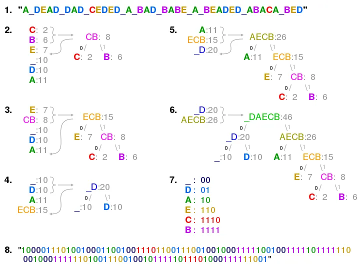
In the 50’s, MIT PhD student David Huffman had to write a paper proving some coding was optimal. He couldn’t figure it out, but extraordinarily, he thought up his own algorithm³ and proved that coding was optimal. Huffman’s professor Robert Fano had previously devised a coding algorithm with⁴ Claude Shannon himself, so when his student showed him a better algorithm, Fano supposedly⁵ canceled class for the rest of the term. In essence, this is the Huffman Coding:

1. Start with the system $\Omega = x_1, x_2,..., x_n$, and $p =$ the probability function.

2. Take $x_i, x_j$ of lowest probability in $\Omega$.

3. Remove $x_i$ and $x_j$ from $\Omega$, and add to $\Omega$ a new character $\chi$, where $p(\chi) = p(x_i) + p(x_j)$.

4. Repeat (1) and (2) until only 1 element remains in $\Omega$.

5. Build a binary tree for which all the leaves are the original members of $\Omega$, and two nodes share a parent if they were replaced by that parent in step (2).

Huffman’s simple $O(n\log(n))$ algorithm finds an optimal symbol-by-symbol coding. There are alternate methods of coding which perform better under certain circumstances, but even where suboptimal, Huffman is quite good.

---

Footnotes

1. Claude Shannon is the father of Information Theory, and an absolute legend. He wrote the book A Mathematical Theory of Communication, which a professor of mine once described as “one of the most important books in science in the last century”. ↩

2. This statistic is from the Wikipedia page on Letter Frequency. ↩

3. David Huffman, A Method for the Construction of Minimum-Redundancy Codes (1952). ↩

4. Fano and Shannon didn’t actually collaborate, rather they independently developed similar algorithms at almost the exact same time. Today these are clumped together as the Shannon-Fano Coding. ↩

5. I’ve only heard this part from one source. ↩